This presentation demonstrates how to assess production loss due to equipment unreliability for equipment arranged in series, parallel, and standby configurations.
Series Configuration
Consider a production system consisting of equipment operating in series.
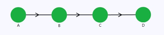
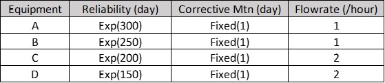
The reliability models, corrective maintenance downtimes, and flowrate (production rate) of each piece of equipment are as shown in Figure 1. From a production performance perspective, it is evident that Equipment A is more reliable than B, B is more reliable than C, and C is more reliable than D.
Rank the Bad Actors according to their Production Loss Contributions
We wish to rank the equipment performance based on its production loss.
The simulation results are obtained through a 365-day simulation with 1000 executions:
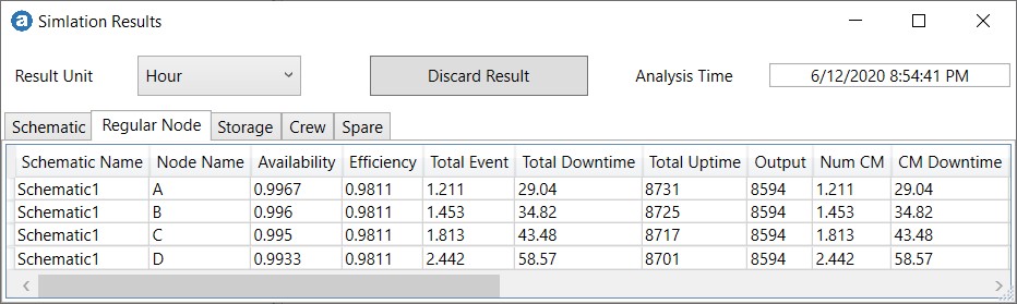
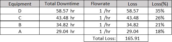
The simulation results in table below provides the downtime of each equipment. The loss due to each equipment can be estimated by multiplying its Total Downtime by its Flowrate.
Note that C and D have a maximum flowrate of 2 units/hour, but their actual flowrates are constrained by equipment A and B maximum flowrates.
Parallel Configuration
Consider a production system with the following construct, where the reliability models, downtime behaviors, and flowrates are the same as the previous example.
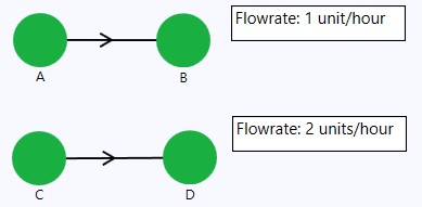
Note that the Flowrate of production line AB is 1 unit/hour, whereas the Flowrate of line CD is 2 units/hour.
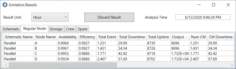
The simulation result is based on a 365-day simulation run with 1,000 executions.
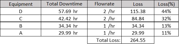
The loss due to each equipment is its downtime multiplied by flowrate.
Standby Configuration
In the above two examples, the losses are calculated based on the fact that the downtime of each item directly contributes to the system loss.
Consider a scenario which involves equipment in standby configuration.
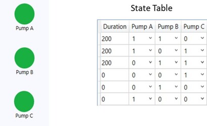
The system operates with a 3-by-2 standby configuration, and switching occurs every 200 hours. If 2 units fail, the system operates with 1 unit, as such it operates with half the load.
The 3 pumps are identical, with Exponential failure distribution (mean = 200 hours), and each takes 50 hours to repair upon failure. The individual flowrate (production throughput) is 1 unit per hour. Therefore, the system flowrate is 2 units per hour.
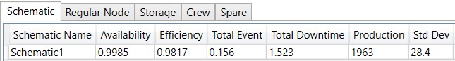
A simulation result is obtained through a 1000-hour simulation with 1000 executions.
At the system level, the Efficiency is 0.9817, and the production is 1963 units (over 1000 hours). We can deduce that the loss is 37 units.
At the equipment level (Regular Node tab):

Note that when an item fails in a standby situation, its failure may not contribute to loss (as long as standby is available). Therefore, we cannot use the downtimes of individual equipment to deduce the total loss as we did in the previous two examples.
Since these 3 pumps are identical, and the total loss is 37 units, we can therefore conclude that each pump contributes a loss of 37/3 units over 1000 hours of operation.
Conclusion
In summary, for series or parallel (or combination) networks, we can use the simulation downtime information of individual items to deduce their loss contribution. For the case of standby systems, first deduce the losses at the system level, then ascribe the losses to each item equally. This works only when all items are identical. In the next article, we will examine loss contribution for standby systems (/RAM Analysis for an Offshore Platform). (/RAM Analysis for an Offshore Platform).
-End-