Introduction

In reliability engineering, a Poisson Process describes events (failures) where inter-arrival times follow an exponential distribution, indicating random failures with a constant failure rate.

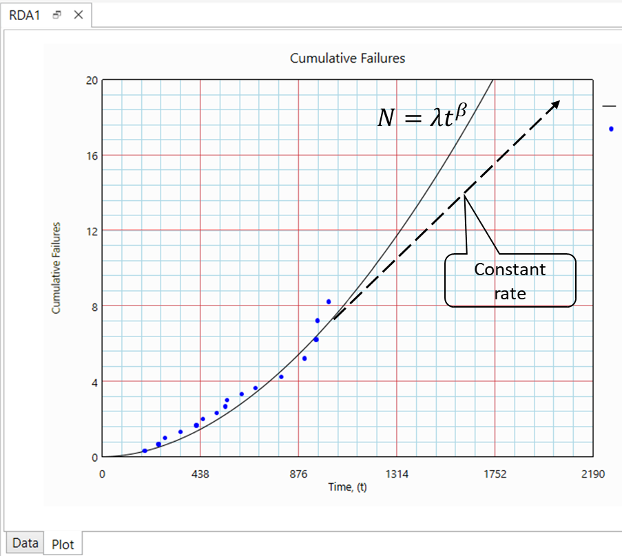
A Non-Homogeneous Poisson Process (NHPP) with Power Law describes events where inter-arrival times follow an exponential distribution, but the failure rate u(t) changes over time according to the Power Law (N=λt^β)

u(t) = dN/dt = λβt^β-1

This model assumes the repairable item has infinitely many failure modes - an assumption that rarely holds true in practice. Analysts must exercise caution when extrapolating results from this model.

Note:

In Life Data Analysis (LDA), the failure rate refers to the number of failures per unit time for a population of non-repairable items.
In Recurring Data Analysis (RDA), the failure intensity describes the number of failures per unit time for a repairable system.

Case Study: Pump System Analysis

The following case study demonstrates this limitation by comparing results from:

Recurring Data Analysis (NHPP with Power Law) applies to the pump system
System Reliability Simulation for the pump system with limited renewable components

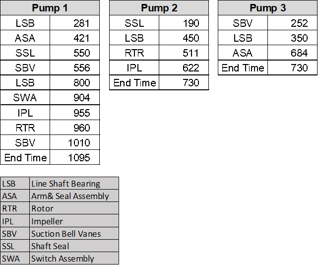
We examine historical failure records for three pumps operating under similar conditions:

Pump 1: 1 year of operation
Pumps 2 & 3: 2 years of operation.

Pump failure records — Figure 1: Historical failure records for 3 pumps

NHPP Approach

Using recurring data analysis (ignoring specific failure modes), we obtain NHPP parameters to predict future failures.

Figure 2: NHPP analysis in Weibull Toolbox (λ=1.484×10^-5, β=1.891)

Cumulative failures curve — Figure 3: Cumulative failures vs time (β>1 indicates increasing failure rate)

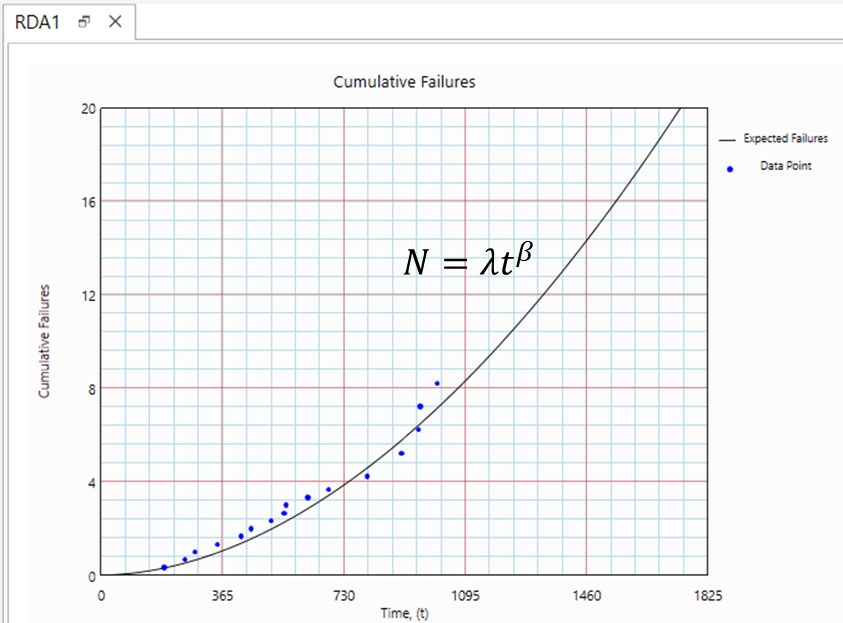
This model estimates the expected cumulative number of failures over time. It can help answer questions such as:

For a new pump, how many failures can I expect in the first 100 day?
For an existing system that is already 3 years old, how many additional failures can be expected if it operates for another 6 months?

Note that our dataset covers a 3-year period. In the second question, we are extrapolating beyond the observed time range. The key consideration is whether the model remains valid beyond the 3-year mark...

Exercising Engineering Judgment in Extrapolating NHPP Model Results.

System Reliability Approach

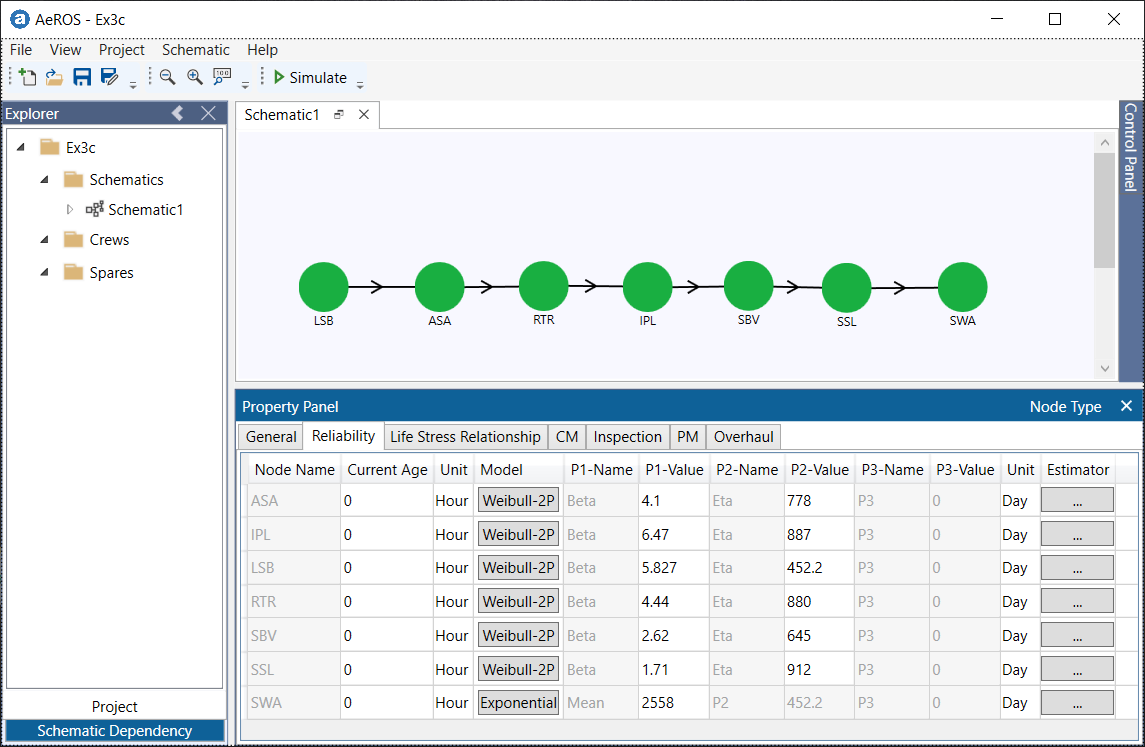
The same system is analyzed using System Reliability approach by constructing the reliability digital twin of the pump system in terms of its components.

This model is used to generate simulated failure sequences to enable direct comparison with the previously established NHPP model.

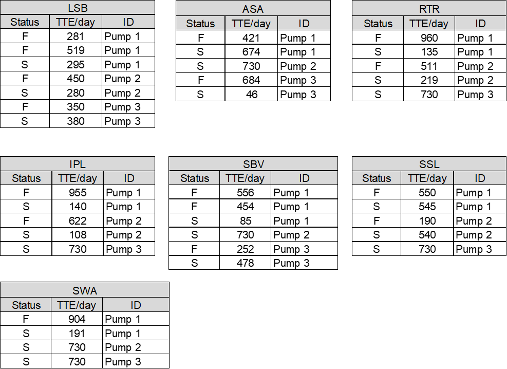
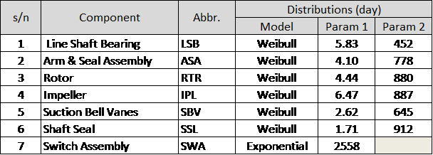
The pump has seven identifiable failure modes (LSB, ASA, RTR, IPL, SBV, SSL, SWA). We model the system reliability in AeROS.

Pump system model — Figure 4: Pump system reliability model

From the historical data (see Figure 1), the Time-To-Failures for each failure mode are extracted as shown in Figure 5:

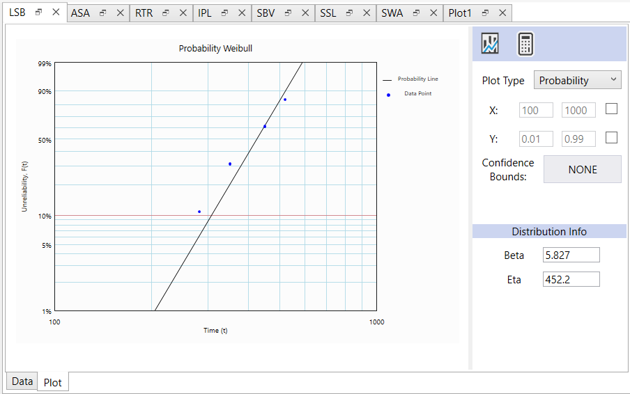
Failure mode data — Figure 5: Time-To-Failure data by failure mode

The datasets are fitted to a distribution model using the LDA module in Weibull Toolbox. Below is the LSB (Line Shaft Bearing) dataset fitted to a Weibull distribution, shown as an example.

LSB Weibull analysis — Figure 6: Weibull analysis for LSB failure mode

The analysis is repeated for the other components. Following is the summary of the pump components’ failure distributions.

Simulation Results

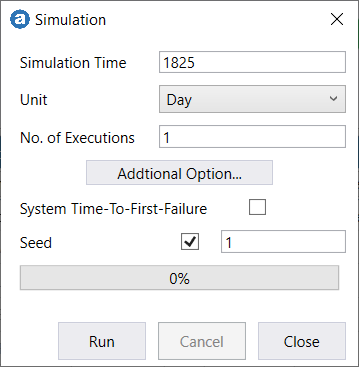
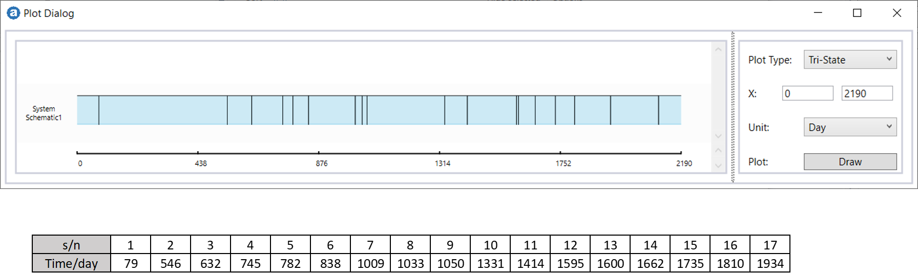
The pump system reliability is modeled in AeROS software and run for a 5-year simulation to generate failure sequences.

System model — Figure 8: Reliability Digital Twin of the Pump

Simulation settings — Figure 9: Simulation parameters

The Tri-State plot shows a sequence of failures over the five-year period.

Failure sequences — Figure 10: Simulated failure sequences

Model Comparison

Two datasets (represented by green and yellow points) were generated using our simulation approach and overlaid onto the previously obtained NHPP model for comparison.

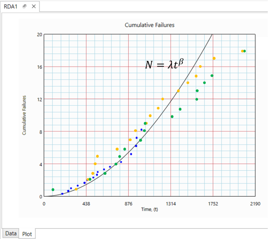
Deviation analysis — Figure 12: System with limited failure modes reaches steady-state (constant failure rate)

In the case of the Non-Homogeneous Poisson Process (NHPP) model, it is assumed that the system has an infinite number of failure modes. When the shape parameter β is greater than 1, the model predicts that failure intensity will continue to increase over time.

However, in simulations using a digital twin with a limited number of failure modes, the failure intensity eventually stabilizes, which aligns more closely with real-world expectations.

The discrepancy grows significantly over long time horizons, making NHPP increasingly deviate from real-world behavior in long-term forecasts.

Key Findings

NHPP assumes infinite failure modes → failure intensity continues increasing (for the case β>1)
Real systems have finite failure modes → failure intensity stabilizes
Discrepancy grows significantly over long time horizons

Conclusion

Recurring data analysis is significantly easier to perform compared to the system reliability approach. In most practical cases, data are not collected at the lowest actionable item level; therefore, recurring data analysis is often the only available option for failure projection. However, analysts should be aware that this approach assumes the (repairable) item has infinitely many failure modes, which is generally not the case. As a result, engineering judgment must be applied when extrapolating results from the model.

related_articles

Inventory Management: Forecasting Repairable Spare Requirements

Applying Recurring Data Analysis: A Use Case Example

- End -