Introduction
When a new reliability test produces only a few failures, analysing those observations alone can give an unstable Weibull shape estimate. Bayesian analysis provides a structured way to combine the new evidence with relevant historical knowledge. This article uses generated data to illustrate the process in FreeWeibull.com.
An Illustrative Supplier Monitoring Example
Assume a supplier continues to provide the same type of component. A previous test produced 20 failures. A later sampling test produced only three failures at 60, 100 and 170 hours. Based on product knowledge and the expected failure mechanism, the engineer judges that the Weibull shape parameter should remain broadly consistent, while allowing the characteristic life to be estimated from the new evidence.
The datasets in this article are generated solely for illustration. In a real application, the relevance of the historical population must be established before it is used as prior information.
Historical Test Results
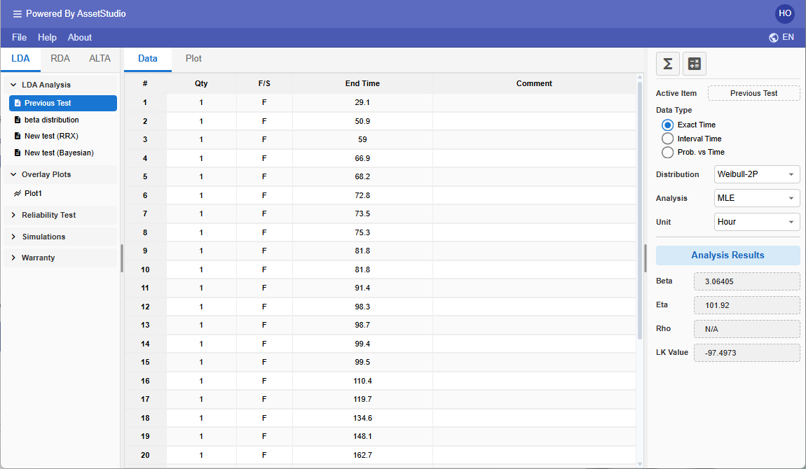
The 20 historical failures are fitted with a two-parameter Weibull distribution using maximum likelihood estimation. The result is β = 3.06405 and η = 101.92 hours. This historical analysis provides both an estimate of β and information about its uncertainty.
Developing a Prior for Beta
Step 1. Fit the historical dataset with a two-parameter Weibull distribution. In this example, the maximum likelihood estimate of β is 3.06405.
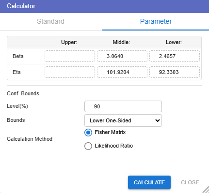
Step 2. Open the Calculator and select the Parameter tab. Choose the Fisher Matrix method, enter a 90 percent confidence level and select Lower One-Sided. The calculated lower bound on β is 2.4657. Repeat the calculation at confidence levels of 80, 70 and 60 percent.
| Confidence level | Lower bound on β | Complementary probability |
|---|---|---|
| 90% | 2.4657 | 10% |
| 80% | 2.6566 | 20% |
| 70% | 2.8034 | 30% |
| 60% | 2.9352 | 40% |
Table 1: Lower one-sided bounds used to construct the prior
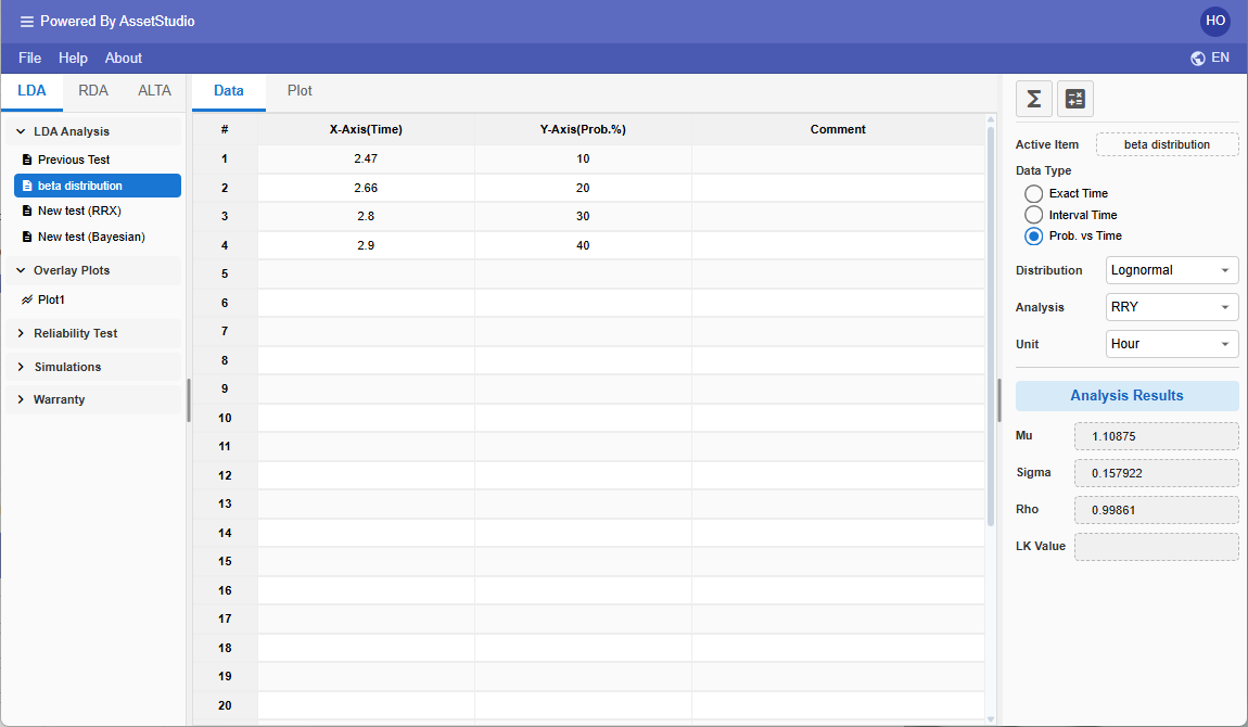
Step 3. Create a Probability vs Time worksheet. Enter the beta bounds on the X-axis and their complementary probabilities on the Y-axis. Select the Lognormal distribution and fit the points using rank regression on Y. The fitted prior has a log-mean of 1.10875 and a log-standard deviation of 0.157922.
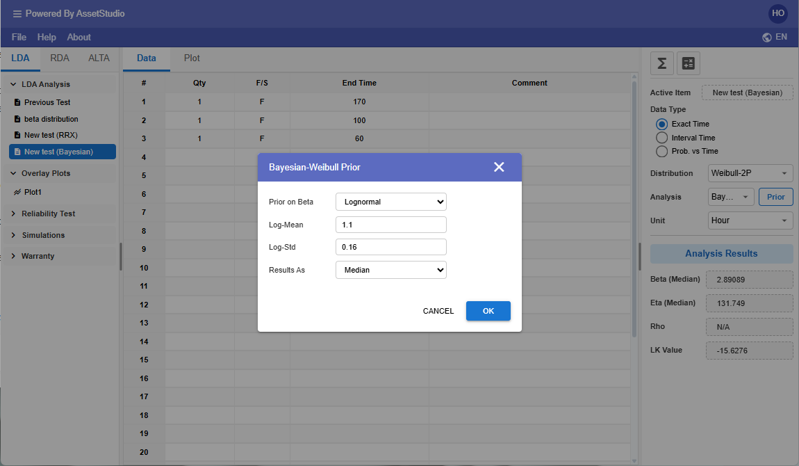
Enter the rounded values 1.10 and 0.16 in the Bayesian prior dialog and report the Bayesian results as medians. The prior is applied to β only; no prior is imposed on η.
Why the Beta Percentiles Follow a Lognormal Distribution
Fisher Matrix confidence bounds for the positive Weibull shape parameter are calculated on a logarithmic scale. The method treats ln(β) as approximately normal. After transforming back to β, the corresponding uncertainty distribution is approximately Lognormal. A 90 percent lower one-sided bound therefore represents the 10th percentile, an 80 percent lower bound represents the 20th percentile, and so forth. Entering the bounds with their complementary probabilities reconstructs the same uncertainty curve. The Lognormal fit is therefore expected; it is not independent evidence that β must have a Lognormal prior.
Using this confidence-bound curve as an informative prior is an illustrative engineering approximation. Frequentist confidence bounds are not Bayesian posterior probabilities, so the relevance of the historical dataset and the sensitivity of the result to the selected prior should still be considered.
Analysing the New Sampling Test
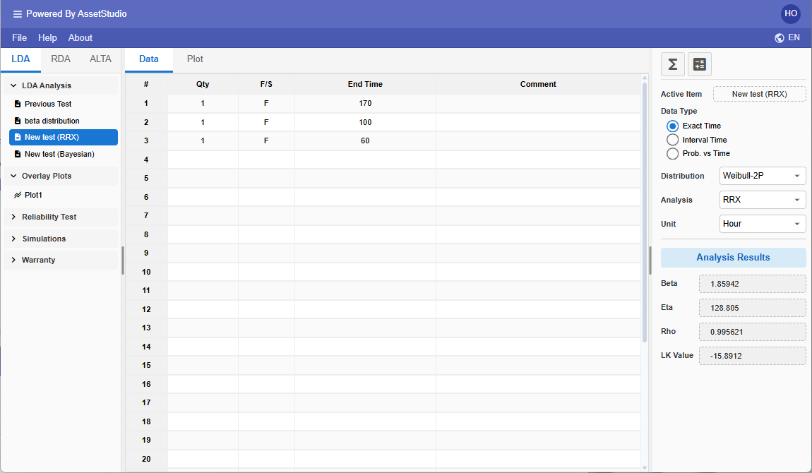
First, the three new failures are analysed by rank regression on X without using the historical information. The estimates are β = 1.85942 and η = 128.805 hours. With only three points, the fitted slope and its confidence bounds are sensitive to the limited sample.
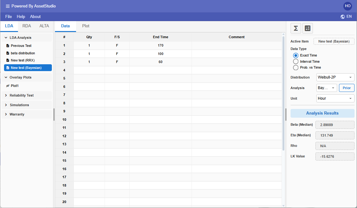
The same three failures are then analysed using the Lognormal prior for β. The posterior median estimates are β = 2.89089 and η = 131.749 hours.
Comparing the Results
| Analysis | Information used | β | η (hours) |
|---|---|---|---|
| RRX | Three new failures only | 1.85942 | 128.805 |
| Bayesian median | Three failures plus prior on β | 2.89089 | 131.749 |
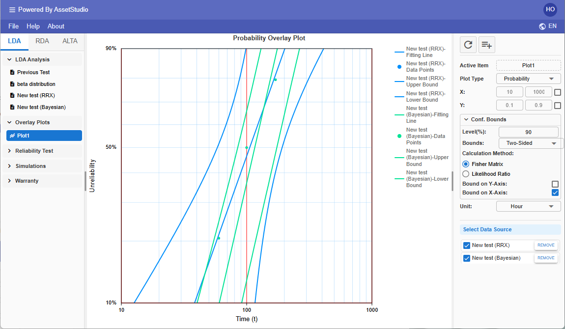
The η estimates are similar, but the β estimates differ substantially. The historical prior stabilizes the shape estimate without forcing the complete historical Weibull distribution onto the new sample. The overlay also shows the reduction in uncertainty associated with incorporating the prior information.
In the overlay, the RRX series uses 90 percent two-sided Fisher Matrix confidence bounds on the time axis. The Bayesian series uses Bayesian bounds; for a Bayesian dataset, FreeWeibull ignores the overlay calculation-method selection.
Using Historical Information Responsibly
A prior should express relevant knowledge, not a preferred answer. Historical information may be suitable when the product, supplier, manufacturing process, operating conditions and failure mechanism remain comparable. If an improvement changes the failure physics, assuming the same β may no longer be justified. Sensitivity studies with wider or alternative priors can show how strongly the conclusion depends on that judgement.
This example demonstrates why Bayesian analysis can be useful when new data are scarce but credible historical information exists. FreeWeibull.com supports Bayesian Weibull analysis alongside conventional life-data methods, making it possible to examine both results within the same workspace.
Try the Bayesian Life Data Analysis module at FreeWeibull.com and view the Bayesian user guide.
- End -