In this article, I will briefly explain how the gamma value is solved when you are fitting a dataset to a 3-Parameter Weibull (3P-Weibull), so that you have enough knowledge to decide whether you should avoid this analysis.

I will also provide an example that demonstrates an appropriate use case of the 3-Parameter Weibull distribution.

3-Parameter Weibull

Beta (β), also known as shape parameter, is a positive value that governs the rate at which the failure rate changes over time. If β < 1, the failure rate decreases over time, indicating the population is getting more stable (in terms of failure) as it ages. If β = 1, the failure rate is constant, and if β > 1, the failure rate increases over time.

Eta (η), also known as characteristic life, represents the time at which 63.2% of the population fails.

Gamma (γ) is a time-shift term used to modify the original 2-Parameter Weibull distribution. If γ = 0, the 3-Parameter Weibull reduces to a 2-Parameter Weibull distribution.

A positive γ means that the population cannot fail before t = γ. From reliability perspective, this is a desirable attribute.

What if the γ is negative? The item from this population can start to fail from a negative time! Note that in reliability engineering, we are only interested in the positive time domain.

If you have no knowledge of the gamma value, stick to the 2P-Weibull

Fitting failure data to a 3-Parameter Weibull

As a reliability engineer, the main reason to use 3P-Weibull for your dataset is that you believe that a 'no failure time', (positive gamma), exist in your population, and you hope that the analysis can tell you this value.

Consider the following two time-to-failure (hours) datasets (generated using Monte-Carlos simulation from 2P-Weibull with the same parameter β =9 and η =3600):

• Dataset 1: 3000, 3086, 3322, 3650, 4001
• Dataset 2: 2850, 3503, 3606, 3800, 4000

Both the datasets are fitted with 2P-Weibull using RRX, and followings are the results:

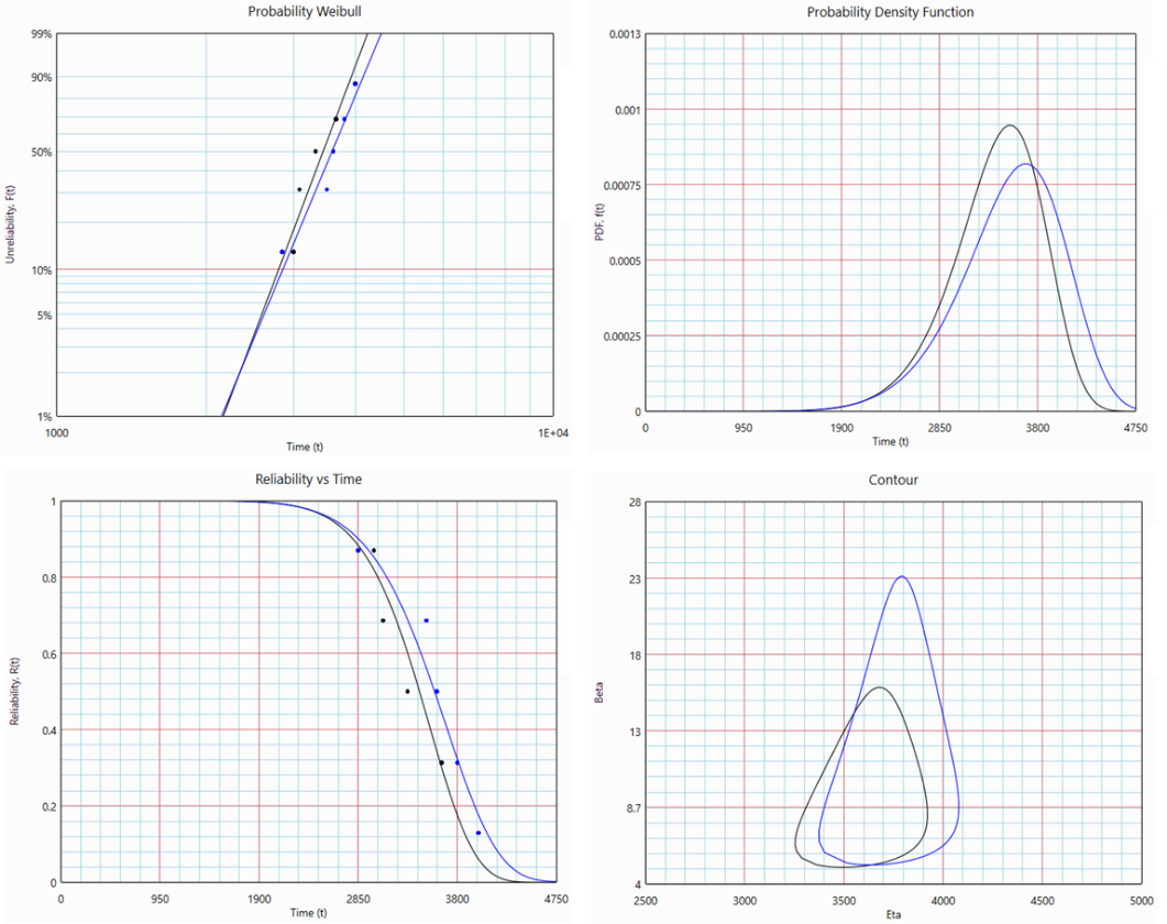
From the contour plots, we can observe that there is no statistical evidence that the two sets are different (i.e., there is a significant overlap between the two contours).

You want to know if γ exist, and so, you proceed with 3P-Weibull analysis. Perhaps you are convinced that it is not possible to fail within the first 1000 hours.

Note that you are expecting a "positive" γ.

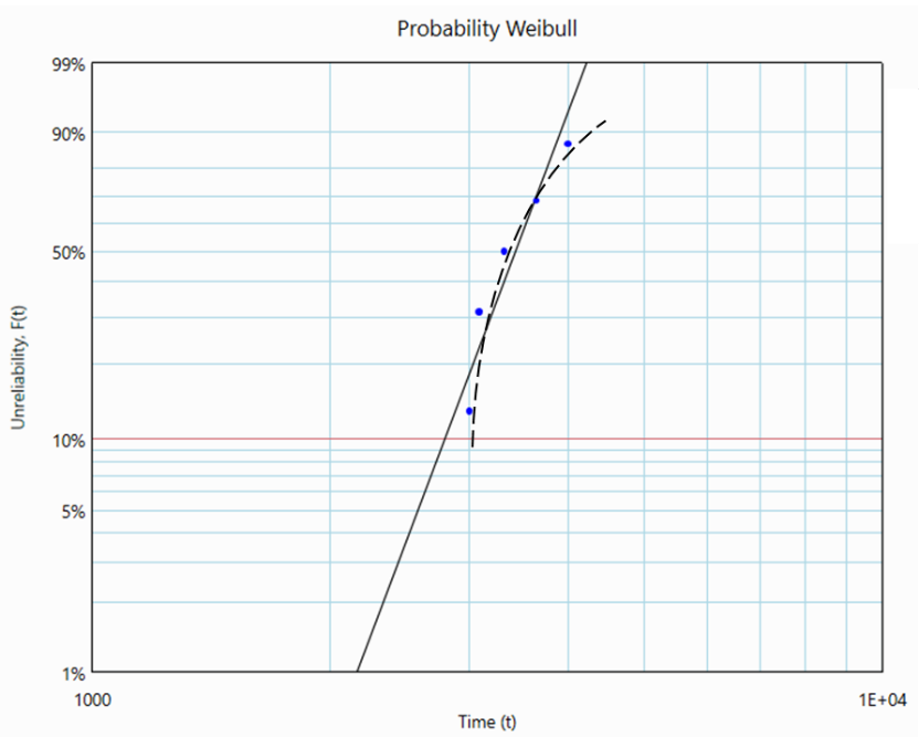
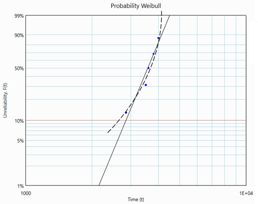
Now, let me explain how γ is calculated with Dataset 1: 3000, 3086, 3322, 3650, 4001

The points are plotted on the Probability-Weibull graph. A 2P-Weibull line regresses along these points. Notice that the points form a curvature facing 'downward' as indicated in Figure 2.

By reducing all the values (times to failure) in the dataset by an appropriate constant (i.e., γ), we can remove the curvature. Let's subtract 2965 from all values in Dataset 1.

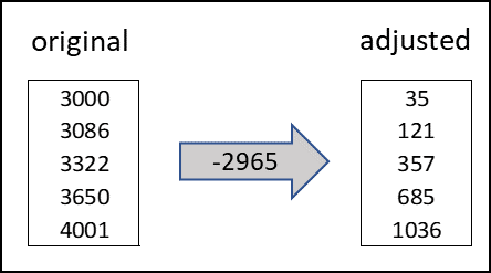
Now we plot these 'adjusted' points on the Probability-Weibull graph.

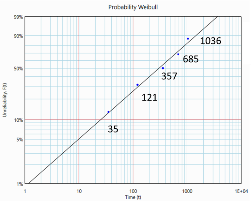
The γ value is 2965 hours- the software search for a gamma value such that the adjusted dataset does not form a curvature.

The β and η are now 0.7611 and 485.8 (hours) respectively (based on the new straight line formed). We have just fitted the original dataset with a 3-Parameter Weibull.

Now, let us proceed to analyze Dataset 2: 2850, 3503, 3606, 3800, 4000. We would expect that the gamma value to be close to that of Dataset 1 (2965). Since smallest failure point for Dataset 2 is 2850, it should be somewhere below 2850.

Dataset 2 is fitted to a 2-parameter Weibull:

To 'straighten' the data points, a negative γ value is required. To form the best possible straight line, the γ value is -582,112 hours!

The corresponding β and η are 1,427 hours and 585,866 respectively!

We ended up with a negative γ—how should we interpret that? On top of that, the β value is extremely large, exceeding 50!

Side note: A large β means that the failure rate increases very sharply when the age is approaching η value. Personally, I would consider other distributions, like Normal or Lognormal if the β is greater than 20.

These two datasets were generated using a Monte Carlo simulation with a 2-parameter Weibull distribution. While no location parameter (γ) was originally included, one can always estimate γ by fitting a 3-parameter Weibull model.

However, when working with real-world data—whether from lab tests, field observations, or simulated datasets—there’s a 50% chance your data will exhibit a downward curvature (and a 50% chance of an upward curvature). In the case of a downward trend, you might obtain a plausible positive γ. Otherwise, you could end up with a nonsensical negative γ.

Given the mathematical nuances (or perhaps madness) behind this analysis, should you trust the estimated γ—even if it appears reasonable (e.g., falling between 0 and the smallest value in your dataset)?

What if we switch from regression to maximum likelihood estimation (MLE) for the 3-parameter Weibull? Without delving into technical details, I’ll simply note that MLE often produces even more absurd results!

Closing Example: A Practical Use Case for the 3-Parameter Weibull

Consider a scenario where you need to model the lead time for spare part arrivals from a supplier to support simulation analysis. Below is the historical lead-time data (in days):

Historical lead-time data (day): 30, 30, 30, 30, 31, 31, 35, 36, 42

You know that the minimum lead time—accounting for administrative processing and shipping—is 27 days. This physical constraint implies no value can fall below 27 days, making it an ideal candidate for the location parameter (γ) of a 3-parameter Weibull distribution.

Steps to Fit the 3P-Weibull:

1. Adjust the dataset by subtracting γ = 27 days:

   [3, 3, 3, 3, 4, 4, 8, 9, 15]

2. Fit the adjusted data to a 2-parameter Weibull (β, η):

   • Shape parameter (β) = 1.64
   • Scale parameter (η) = 6.5 days

3. Final 3P-Weibull distribution:

   • β = 1.64, η = 6.5 days, γ = 27 days

This approach ensures the distribution respects the real-world constraint (γ = 27) while accurately modeling the variability in lead times.

We cannot expect that one could extract a gamma value through fitting the data to a 3P-Weibull (i.e., mathematically). Gamma should be a quantity that is known to the analyst. If you have no knowledge of the gamma value, stick to the 2P-Weibull.

When something is too good to be true it usually is...