Introduction

In Printed Circuit Board Assemblies, solder joint failures can occur due to fatigue caused by temperature cycling. Norris-Landzberg model has been used to model fatigue failure in solder joints due to repeated temperature cycling as the device is switched on and off.

This article presents an analysis of accelerated test data for lead-free solder joint low-cycle fatigue using the Norris-Landzberg model. We derive the model parameters through the General Log-Linear (GLL) relationship, implemented in AssetStudio’s Weibull Toolbox software.

Norris-Landzberg model

The number of cycles to failure in the Norris-Landzberg model is represented as:

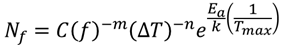
where:

N_f: number of cycles to failure
C: coefficient
f: cycling frequency (cycles/day)
ΔT: temperature range during a cycle (K)
T_max: number of cycles to failure
E_a: maximum temperature during each cycle (K)
K (= 8.617 x 10^-5 eV/K): activation energy (eV)
m, n: Boltzmann's constant

The Norris-Landzberg model accounts for three key stresses that affect solder joint fatigue life:

Cycling frequency, f - Modeled using an Inverse Power Law (IPL) relationship
Temperature range, ∆T - Also following an Inverse Power Law (IPL) relationship
Cycle maximum temperature, T_max - Governed by an Arrhenius relationship

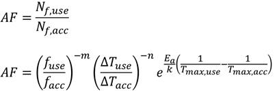
Acceleration Factor (AF), the ratio of Life at use-stress to Life at accelerated-stress, can be expressed as:

General Log-Linear model

The General Log-Linear (GLL) model expresses characteristic life (L) under three stress conditions as:

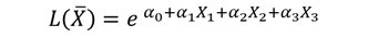
Here, L can represent any distribution percentile - η (Weibull scale parameter) or median life (Lognormal).

To align with the Norris-Landzberg model, we apply the following transformations:

X₁=ln(f)

X₂=ln(∆T)

X₃=1/T_max

These transformations yield:

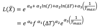
By comparing it with the Norris-Landzberg model equation, the parameter relationships can be derived:

C = e^α0
m = -α₁
n = -α₂
E_a/K =α₃

Example

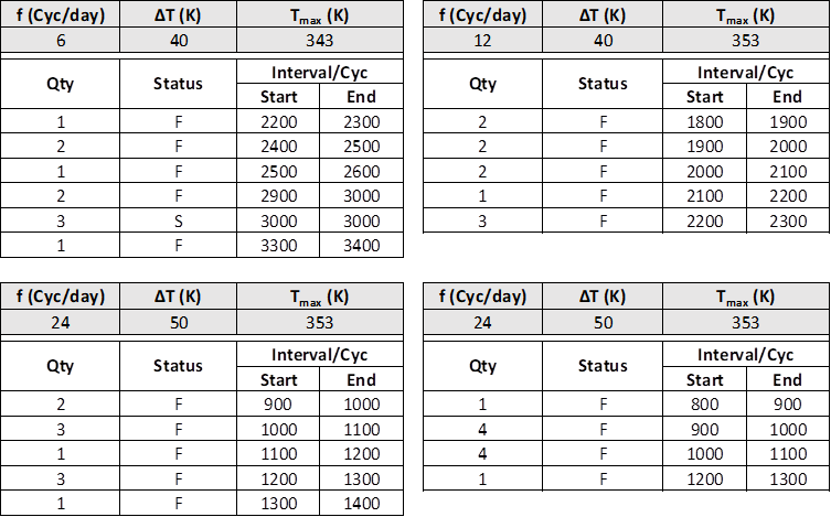
The following is an accelerated life test using GLL life-stress relationship with 3 stresses for a particular lead-free solder joint type. The figure shows the results of thermal cycling test with different stress level settings. For a 3-stresses model, the minimum number of experiments is 4 (because there are 4 unknowns to be solved). Each test uses 10 units. The units are inspected every 100 cycles.

Figure 1, Thermal cycling test results of 4 experiments, each with unique accelerated stress settings

The underlying distribution is assumed to be lognormal. The stress model for f (cycling frequency) and ΔT (temperature range during cycling) are set to Inverse Power Law, and T_max is set to Arrhenius model as shown on the right panel in below (figure 2).

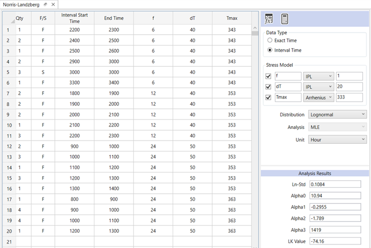
Figure 2, The dataset is entered into Weibull Toolbox ALTA module.

The analysis results can be used to derive the parameters of Norris-Landzberg model:

C = e^α0 = 56,387
m = -α₁ = 0.2955
n = -α₂= 1.789
E_a/K = α₃ = 1419

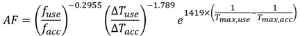
Hence, the acceleration factor for this lead-free solder joint temperature cycling life is:

Assuming you conducted an accelerated life with the following settings:

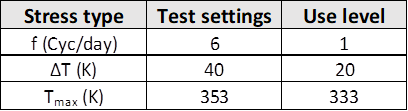
and further assume that you obtain the mean Life of 1500 (cycles) from your dataset.

From the above formula,

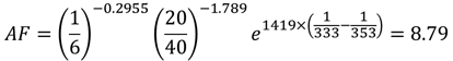
The projected mean life is 1500 x 8.79 = 13,185 cycles at use-level stress.

Conclusion

The article demonstrates how quantitative accelerated life test analysis can be used to calculate the Norris-Landzberg model for solder joint open circuit failure resulting from thermal cycling conditions. Similar process can be applied to other commonly used accelerated life stress test for electronic devices like Hallberg-Peck model.

Reference

K. C. Norris and A. H. Landzberg, "Reliability of controlled collapse interconnections," IBM Journal of Research and Development 13, no. 3 (1969): 266–271.

-End-