Resources Center - Life Data Analysis for product with multiple failure modes

Multiple failure modes are the different ways in which a particular unit might fail. Consider a population of units can fail due to failure modes A, B and C. The observed failure time is the minimum of these individual potential failure times. Reliability model for the unit is reconstructed with A, B and C in series.

This presentation shows the procedure for analysing products with multiple failure modes, and compare with the analysis where failure modes information is ignored. The product reliability model is then obtained by combining the reliability of each failure modes in series.

The dataset used in this presentation is obtained from Meeker, Escobar (Statistical Methods for Reliability Data).

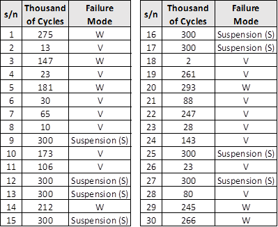
An electric component that has two failure modes, wear-out, W and voltage surge, V.

Resources_MultiFM_Table1 — Table 1, Time-to-Failure with failure mode. W indicates wear out failure, and V indicates voltage surge failure.

Analyzing non-repairable item with multiple failure modes.

Supposing you are interested only on the wear out failure mode (W), those items that failed due to voltage surge (V) are considered as Suspension (S).

Similarly, if you are interested only on the voltage surge failure mode (V), those items that failed due to wear out failure mode (W) are considered as Suspension (S).

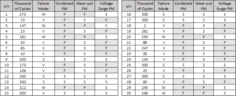
Two additional columns are added in the following table to indicate the Failure/Suspension status for the corresponding failure mode of interest.

Resources_MultiFM_Table2 — Table 2, Time-to-Failure dataset with corresponding failure mode: Combined (Ignore) FM, Wear-out FM and Voltage Surge FM.

We fit all three datasets with Weibull distribution and overlay the plots on the same graph.

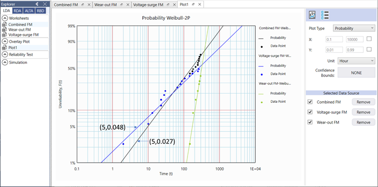
Resources_MultiFM1 — Figure 1, Probability Weibull overlay plot.

The blue and green lines are models for Voltage Surge and Wear-out failure mode respectively. The black line is the model for Combined failure mode (or ignore failure modes).

Resources_MultiFM2 — Figure 2, Unreliability vs Time overlay plot.

The item unreliability at t = 5 (Thousand Cycles), can be obtain from the Combined failure mode line: Q(5) = 0.027 (see Figure 1)

=> R(5) = 0.973

Note that this item consists of 2 Failure Modes (V and W). However, from V failure mode, the unreliability Q(5) = 0.048 (see Figure 1)

=> R(5) = 0.952

If we have a system with 2 components (or failure modes) in series, the system reliability at time t, is always less than any of the components at time t.

We therefore should analyze at failure mode levels (or component levels) whenever possible.

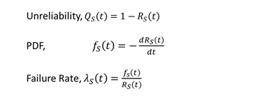
We have analyzed at the failure mode levels. To obtain the system level Q_S(t)…

Since, R_s(t) = R_M(t) * R_V(t)

Q_S(t) = 1 - [(1 - Q_M(t)) * (1 - Q_V(t))]

Weibull-Toolbox RBD module allows you to re-construct the item reliability model in terms of the failure mode V and W connected in series.

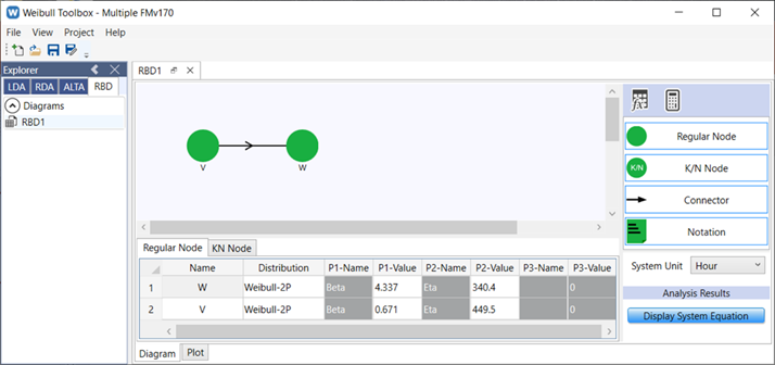
Resources_MultiFM3 — Figure 3, The item reliability is modeled with failure mode V and W, in series.

Based on the system equation:

R_s(t) = R_M(t) * R_V(t),

the other reliability metrices can be derived with the following equations:

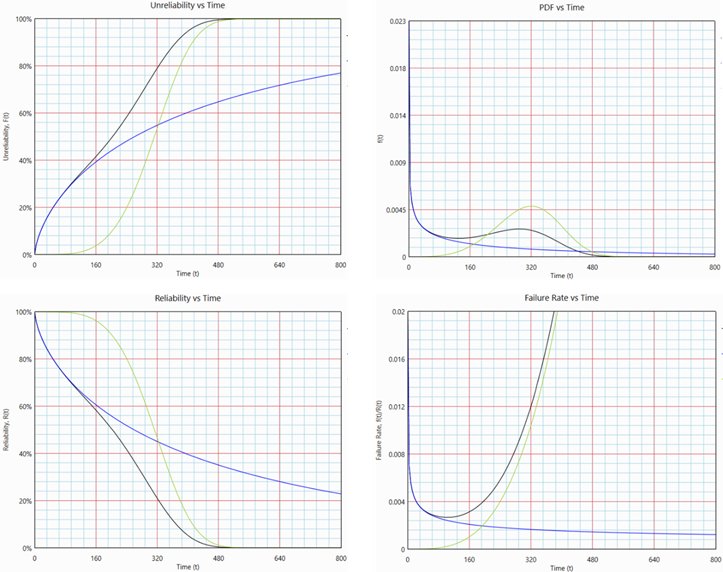
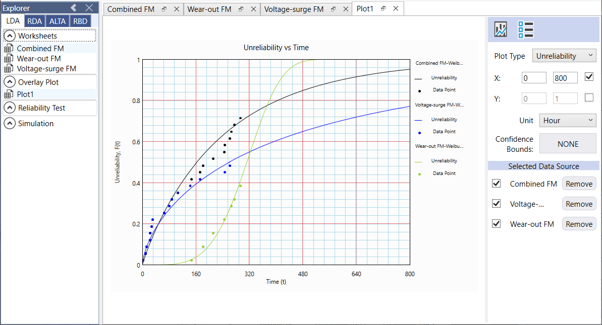
Resources_MultiFM5 — Figure 4, The black, blue and green lines represent the system (item), V and W failure mode model respectively.

Reader can compare the item Unreliability curve in Figure 4 with the item Unreliability curve in Figure 2.

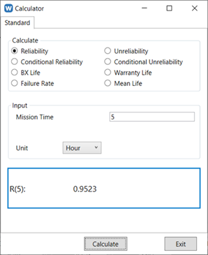
Standard reliability metrices of the system can be queried using the built-in Calculator.

Summary

This example demonstrates the procedure for analyzing non-repairable item with multiple failure modes. The unit reliability is then reconstructed using series-system, and provides more insight to it reliability behavior.

However, this analysis is possible only if failure analysis is performed on every failed component.

-End-